Introduction

This blog covers the theoretical framework behind Gradient Boosting Tree and its implementation in Python without using any libraries that directly implement it.

Motivation

See the previous blog on Random Forest.

What is Gradient Boosting Tree?

Similar to Random Forest, Gradient Boosting Tree (GBT) also consists of a collection of decision trees. However, unlike Random Forest, which trains those trees independently, GBT trains its trees sequentially. The next tree uses the residuals of the previous tree as its target variable instead of the original labels in classification tasks. This means that classification tasks for GBT are treated as regression problems since residuals are used as the target variable.

When constructing the decision tree, the loss is calculated using residuals instead of labels. Below, we provide an example of how this works for classification tasks. For a visual demonstration of the algorithm, refer to StatQuest. Note that the video omits details on how the decision tree is constructed. In the example below, MSE loss is used.

To find the optimal split point, each value of all features is considered. The loss of each split is calculated using the weighted MSE of the sub-groups. The predicted value of each sub-group is the mean of all residuals in that group.

---

Implementation

The gbt Function

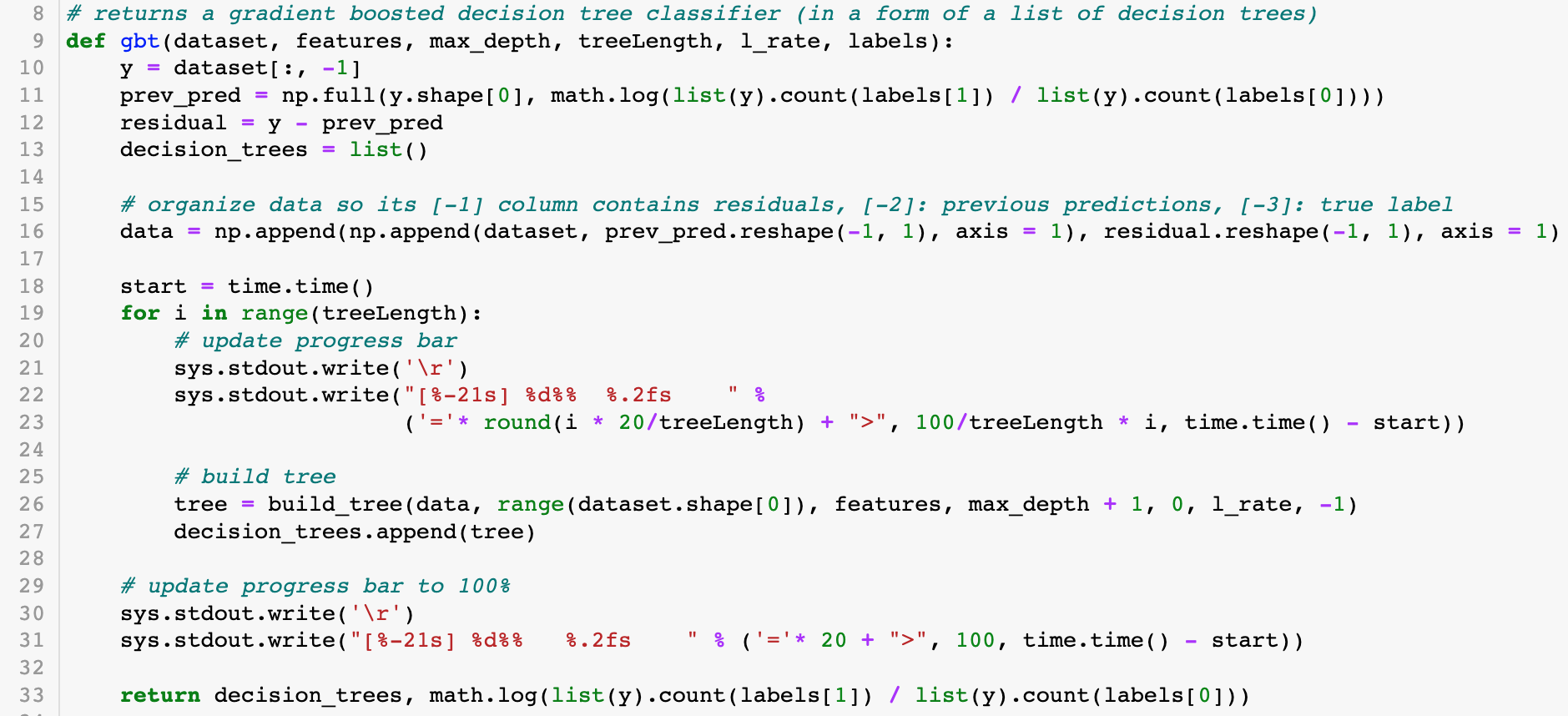
The core of the program is the gbt function:

This function calls the build_tree function a specified number of times (treeLength) and updates a progress bar accordingly. The trees returned from build_tree are stored in a list named decision_trees.

---

The build_tree Function

The steps to build a tree are as follows:

1. Find optimal split using MSE loss (lines 47–55).
2. Initialize the node and fill in the decision boundary (lines 58–62).
3. Construct left and right sub-trees under certain conditions (lines 66–69).
4. Find the output of the leaf node and update predictions and residuals (lines 72–78).

Key Differences from Random Forest

• The loss function for finding the optimal split uses MSE since GBT treats classification as a regression problem.
• Updates at leaf nodes include recalculating predictions and residuals.

Loss Function

For GBT classification tasks, the Mean Squared Error (MSE) is used to find the optimal split:

An example:

• Residuals: 0.1, 0, -0.1
• Predicted value: 0
• MSE: \(\frac{(0.1 - 0)^2 + (-0.1 - 0)^2 + (0 - 0)^2}{3} = \frac{1}{150}\)

---

Node Initialization and Split

After finding the optimal split point, the node is initialized, and the split point is stored.

Conditions for Extending Sub-Trees:

• Both left and right sub-groups must have positive lengths.
• The weighted MSE of the split must be less than the MSE of the current node.

Output Calculation for Leaf Nodes

At leaf nodes, the output is computed as:

Predictions are updated using:

Residuals are updated using:

---

Making Predictions

To make a prediction for (x), the predict function passes (x), all trained trees, initial predictions, and the learning rate. Each tree’s output is summed and passed to a sigmoid function to generate probabilities. Predictions are made using a threshold of 0.5.

---

Cross-Validation

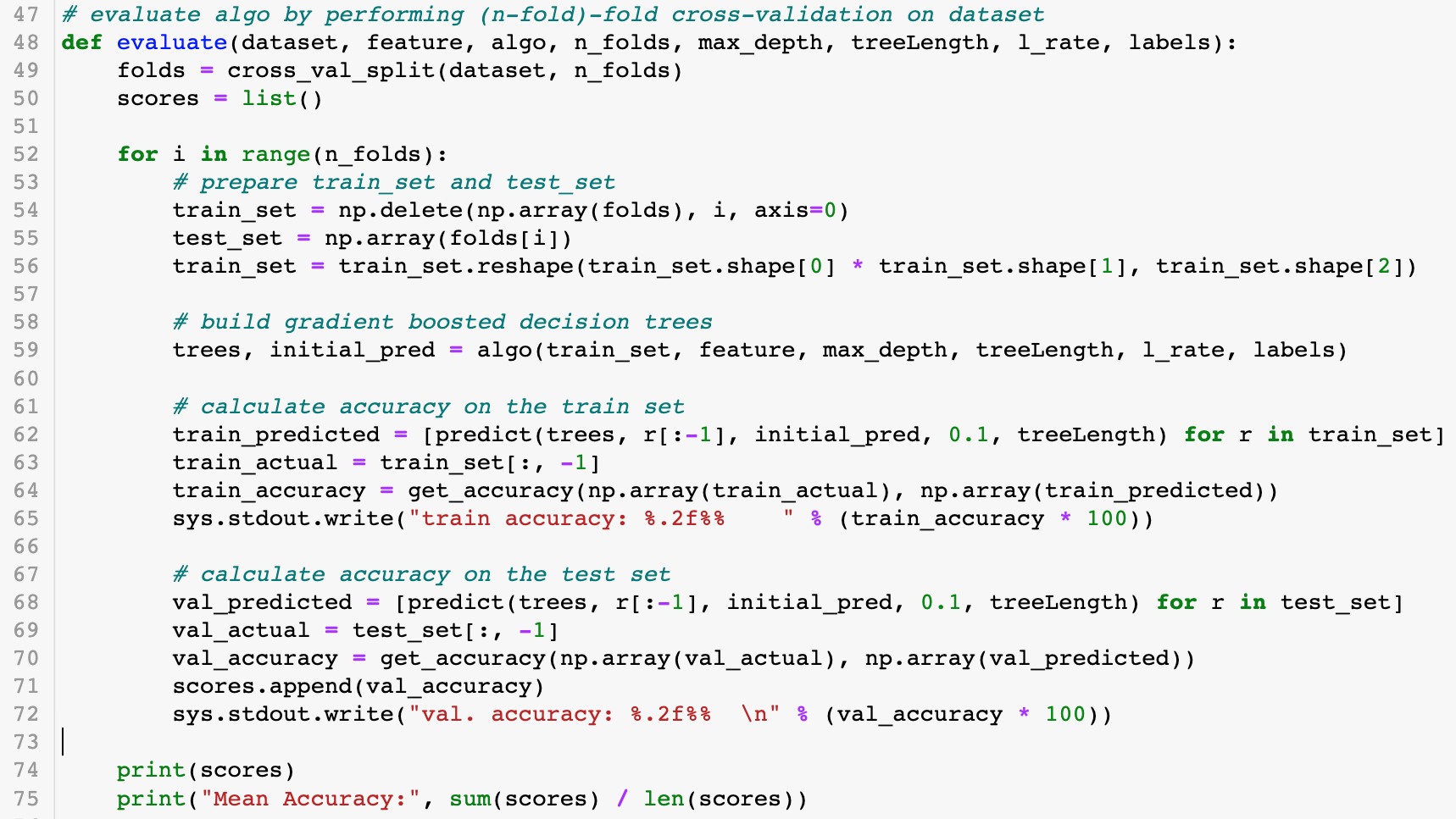
The eval function performs n-fold cross-validation on the dataset:

---

Results

Using 10-fold cross-validation, an accuracy of 86% was achieved on the validation set:

---

Parameter Tuning

GBT requires setting three hyperparameters:

1. Max Depth
2. Number of Trees
3. Learning Rate

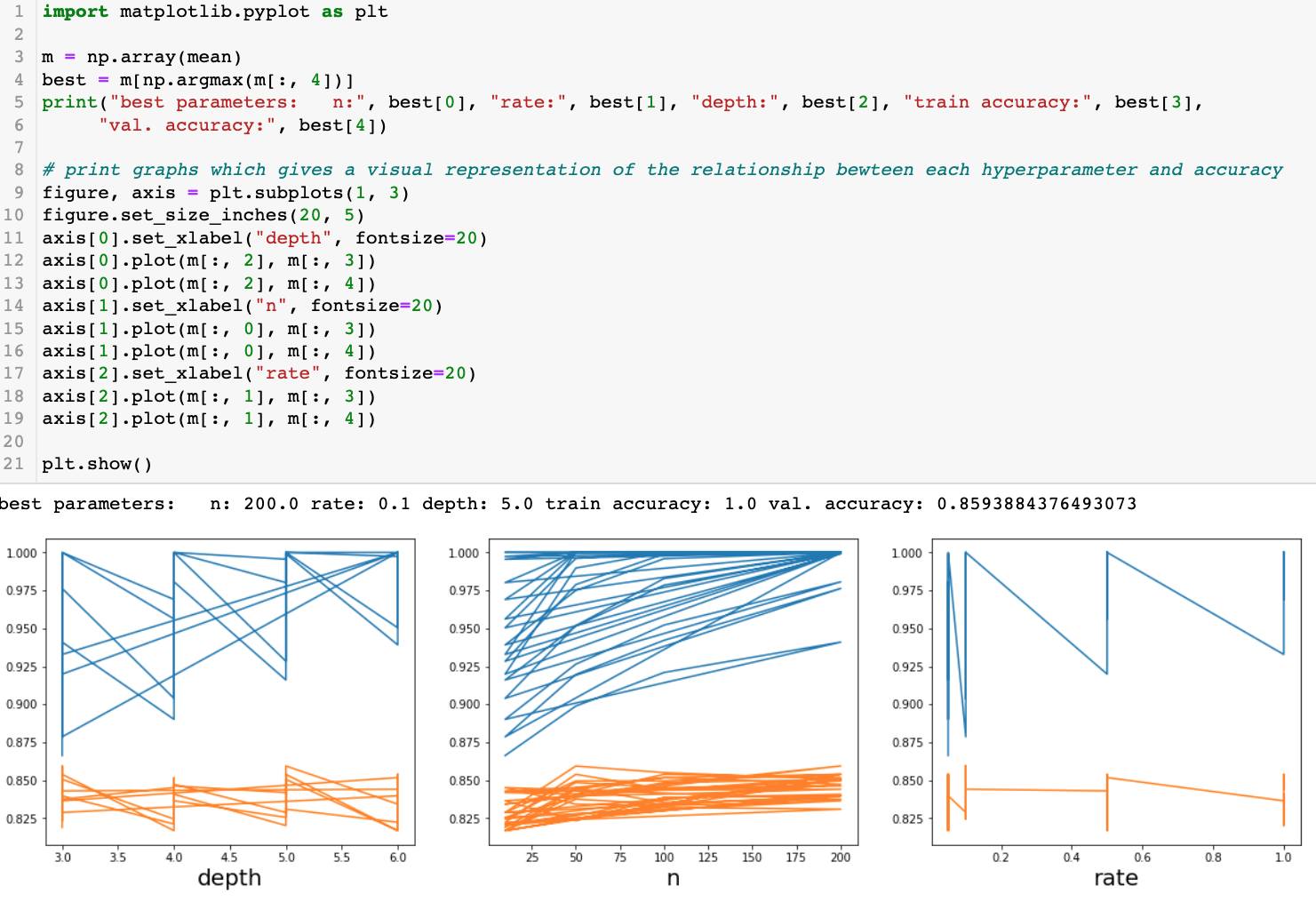
To find the best combination, all possible values are tested using the sklearn library:

Results showed that 200 trees with a max depth of 5 and a learning rate of 0.1 achieved the best validation accuracy (85.94%), slightly lower than the custom implementation.

---

Implementation

For full implementation details, see the GitHub repository.